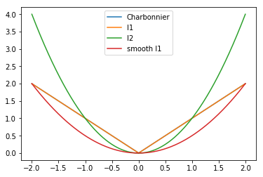
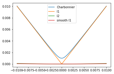
Loss Functions¶

L2 & L1 Loss¶

L2 - MSE, Mean Square Error¶

\[\begin{split}&L_2(x)=x^2\\ &f(y,\hat{y})=\sum^N_{i=1} (y_i-\hat{y_i})^2\end{split}\]

Generally, L2 loss converge faster than l1. But it prone to over-smooth for image processing, hence l1 and its variants used for img2img more than l2.

L1 - MAE, Mean Absolute Error¶

\[\begin{split}&L_1(x)=|x|\\ &f(y,\hat{y})=\sum^N_{i=1} |y_i-\hat{y}_i|\end{split}\]

** MAE seems better than MSE in image generation task, such as super-resolution

Smooth L1¶

\[\begin{split}\text{smooth L}_1(x)= \begin{cases} 0.5x^2 & if |x|<1 \\ |x|-0.5 & otherwise \end{cases}\end{split}\]

\[\begin{split}&f(y,\hat{y})= \begin{cases} 0.5(y-\hat{y})^2 & \text{if } |y-\hat{y}|<1 \\ |y-\hat{y}|-0.5 & otherwise \end{cases}\end{split}\]

Charbonnier Loss¶

LapSRN: Fast and Accurate Image Super-Resolution with Deep Laplacian Pyramid Networks

\[\text{Charbonnier Loss}(x) = \sqrt{x^2+\epsilon^2}, where \epsilon = 1\times 10^{-3}\]

middle_img

Regression Loss Functions¶

MSE - Mean Squared Error¶

\[f(y,\hat{y})=\dfrac{1}{d}\sum^N_{i=1} (y_i-\hat{y}_i)^2\]

MAE - Mean Absolute Error¶

\[f(y,\hat{y})=\dfrac{1}{d}\sum^N_{i=1} |y_i-\hat{y}_i|\]

MSLE - Mean Squared Logarithmic Error¶

\[f(y,\hat{y})=\dfrac{1}{d}\sum^N_{i=1} (log(y_i+1)-log(\hat{y}_i+1))^2\]

Cosine Proximity¶

\[\newcommand{\vect}[1]{\boldsymbol{#1}} f(\vect{y},\hat{\vect{y}})=-\dfrac{\vect{y} \cdot \hat{\vect{y}}}{||\vect{y}||_2 \cdot ||\hat{\vect{y}}||_2}= \dfrac{\Sigma^n_{i=1}y_i\cdot\hat{y}_i}{\sqrt{\sum^n_{i=1}y_i^2}\cdot\sqrt{\sum^n_{i=1}\hat{y}_i^2}}\]

Binary Classification Loss Functions¶

Binary Cross-Entropy¶

\(\hat{y}\) is prediction, y is ground truth

\[f(y,\hat{y})=-\dfrac{1}{n}\sum^n_{i=1}[y_i log(\hat{y}_i)+(1-y_i) log(1-\hat{y}_i)]\]

Hinge Loss¶

max-margin objective

\[f(y,\hat{y})=\dfrac{1}{n}\sum^n_{i=1}max(0,m-y_i\cdot\hat{y}_i)\]

Squared Hinge Loss¶

\[f(y,\hat{y})=\dfrac{1}{n}\sum^n_{i=1}(max(0,m-y_i\cdot\hat{y}_i))^2\]

Multi-Class Classification Loss Functions¶

Multi-Class Cross-Entropy Loss¶

\[f(y,\hat{y})=-\sum^M_{c=1}y_c log(\hat{y}_c)\]

M: total number of class

Softmax Loss, Negative Logarithmic Likelihood, NLL¶

Cross Entropy Loss same as Log Softmax + NULL Probability of each class

\[f(s,\hat{y})=-\sum^M_{c=1}\hat{y}_c log(s_c) \]

\(\hat{y}\) is 1*M vector, the value of true class is 1, other value is 0, hence

\[f(s,\hat{y})=-\sum^M_{c=1}\hat{y}_c log(s_c) = -log(s_c)\]

, where c is the true label

Kullback Leibler Divergence Loss¶

=MLE (Max likelihood estimation) probability distribution

\[\begin{split}f(y_i,\hat{y}_i)& =\dfrac{1}{n}\sum^n_{i=1}D_{KL}(y_i||\hat{y}_i)\\ & =\dfrac{1}{n}\sum^n_{i=1}[y_i\cdot log(\dfrac{y_i}{\hat{y}_i})]\\ & =\dfrac{1}{n}\sum^n_{i=1}(y_i\cdot log(y_i))-\dfrac{1}{n}\sum^n_{i=1}(y_i\cdot log(\hat{y}_i))\end{split}\]